Inline Interactivity in Jupyter using MyST - Herramientas de ciencia de datos

The JupyterLab MyST extension allows you to have MyST renderer in your markdown cells that includes interactivity and inline-evaluation.

This is done through the {eval}`1 + 1` role, which results in 2. The extension can also access variables in the kernel.

import numpy as np
array = np.arange(4)

🛠 In Exercise 1 replace each ??? with an {eval} role for the correct expression

Solution to Exercise 1

This is done through using MyST syntax: {eval}`array.sum()` and {eval}`array.max()`, respectively.

import ipywidgets as widgets

cookiesSlider = widgets.IntSlider(min=0, max=30, step=1, value=10, description="Cookies: ")
cookiesText = widgets.BoundedIntText(
    value=10,
    min=0,
    max=30,
    step=1,
)
widgetLink = widgets.jslink((cookiesSlider, 'value'), (cookiesText, 'value'))

caloriesPerCookie = 50
dailyCalories = 2100.

calories = widgets.Label(value=f'{cookiesSlider.value * caloriesPerCookie}')
def fc(n):
    calories.value = f'{n["owner"].value * caloriesPerCookie}'
cookiesSlider.observe(fc)


percent = widgets.Label(value=f'{cookiesSlider.value * caloriesPerCookie / dailyCalories:.1%}')
def fp(n):
    percent.value = f'{n["owner"].value * caloriesPerCookie / dailyCalories:.1%}'
cookiesSlider.observe(fp)

You can also edit this through a slider if you want: IntSlider(value=10, description='Cookies: ', max=30)

Improvements

There is a lot to improve both for formatting (e.g. format the numbering) and for the verbosity of the above code for linking and calculating the widgets. These are probably going to be a combination of a MyST library for working with simple inline widgets and showing numbers, as well as improvements and tweaks to the inline renderers for the mime bundles.

But you can already do things! 🚀

import numpy as np
import matplotlib.pyplot as plt

def plotStocks(line_color = 'b'):
    # Step 1: Predict the stock market, with surprising accuracy:
    data = np.cumsum(np.random.rand(1000)-0.5)
    data = data - np.mean(data)

    stocks = plt.figure(figsize=(10,2))
    ax1 = stocks.add_subplot(111)
    ax1.plot(data, line_color)
    ax1.axhline(c='grey', alpha=0.5);
    plt.axis('off')
    plt.tight_layout();
    plt.close();

    annotated = plt.figure(figsize=(10,2))
    ax1 = annotated.add_subplot(111)
    plt.axvspan(450, 560, color='red', alpha=0.5)
    plt.axvspan(680, 740, color='green', alpha=0.5)
    ax1.plot(data, line_color)
    ax1.axhline(c='grey', alpha=0.5);
    plt.axis('off')
    plt.tight_layout();
    plt.close();
    
    return stocks, annotated

stocks, annotated = plotStocks('r')

If we look at the following stock price for Apple (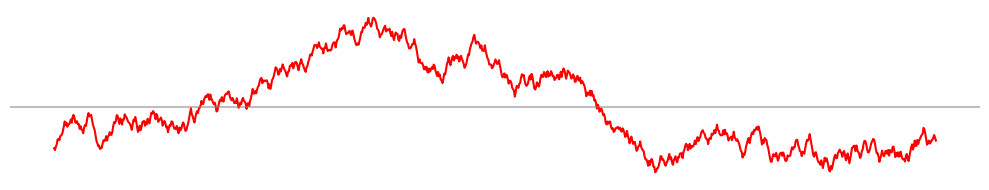) we can see that in 2003, they started selling computers, in the red region and their stock went crazy once the investment paid off (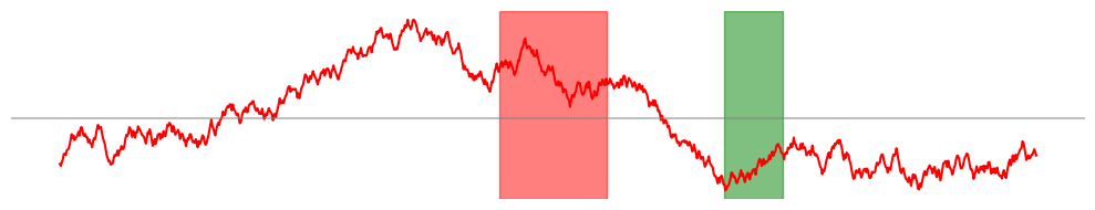).^[1]

from sympy import symbols, expand
x, y = symbols('x y')
expr = x + 2*y
polynomial = x*expr

🛠 Try changing the expr above and then re-execute this cell to see the update!

When we expand the polynomial x \left(x + 2 y\right), we get x^{2} + 2 x y.

from IPython.display import Image, HTML

i = Image(url='https://source.unsplash.com/random/400x50?sunset')

This should be an inline image of a sunset: <img src="https://source.unsplash.com/random/400x50?sunset"/>

text_hover = HTML('<span onmouseover="this.innerText=\'💚\'" onmouseout="this.innerText=\'🎉\'">❤️</span>')

Try hovering over this element^[2]: <span onmouseover="this.innerText='💚'" onmouseout="this.innerText='🎉'">❤️</span>

Footnotes¶

Both the graphs are fake, but pretty cool right!
↩
You may need to set your notebook to trusted to do this!
↩